library(tidyverse)
theme_set(theme_bw(18))Learning objectives
In today’s lab you will…
- Fit a linear model to real world data
- Interpret model coefficients
- Simulate data according to model assumptions and recover parameters
Storms and floods
We’ll begin with an example of the relationship between precipitation and flooding during storms in LA. Save the LA Storm Data CSV to your data/ folder and use it to fill in the following code chunk. Each row in the CSV file contains data from a storm in LA during the last fifteen years. gage_ht is the height of the Los Angeles River at the Sepulveda Dam (in feet) and precip_wk_in is the total precipitation measured during the previous week at the Hollywood Burbank Airport. You can find data like these through USGS and NCEI, respectively.
# Read the CSV file into a data frame

# Create a plot of the gage height and precipitation data
Q1: Which variables did you choose for the x- and y-axis? What does this imply about the data generating process?
In Quarto documents, we can add statistical notation using LaTeX. We’ll fill in the equation below to describe the model.
\[ \begin{align} ??? &\sim Normal(???, ???) \\ ??? &= ??? + ??? \end{align} \]
Fit model
The lm() function fits a linear regression model to data. It has two important parameters: the formula defining the model, and the data frame containing the data.
Once you’ve fit the model, use summary() to see the details, including the coefficients and \(R^2\) value. \(\hat \sigma\) is in there too, but doesn’t print by default. Assign the result of summary() to a variable called storm_summ and try to find the standard deviation from there (hint: it’s an element in that variable).
Q2: What are the estimates for \(\hat \beta_0, \hat \beta_1, \hat \sigma\) ?
Interpret model
Q3: In plain language, describe how you’d interpret \(\beta_0\) and \(\beta_1\). What do they represent?
Let’s also interpret \(R^2\), the measure of model fit. Recall \(R^2\) describes the amount of variance explained by the model. In other words, how much variance did we “explain away” using the model’s prediction line. In equations, it looks like this.
\[ \begin{align} SST &= \sum_i (y_i - \bar y)^2 \\ SSE &= \sum_i (y_i - \hat y_i)^2 \\ R^2 &= \frac{SST-SSE}{SST} \end{align} \]
We can get \(R^2\) directly from the model summary in R, but it’s helpful for your learning to do it a couple times directly, too. Calculate \(SST\), \(SSE\), and \(R^2\) arithmetically in the code chunk below. You can use the coef() function to get the model coefficient estimates, but don’t use residuals().
y_bar <- ???
y_hat <- ???
SST <- ???
SSE <- ???
R2 <- ???
Q4: What’s the difference between \(y\), \(\bar y\), and \(\hat y\)?
Q5: What does the \(R^2\) value tell you about the quality of the model (in plain language)?
Recall that the purpose of a model is to explain variance.
Q6: What’s the estimated value of \(\hat \sigma\) for the model? What’s the value of \(\sigma\) for the response variable itself? Say you needed to predict Los Angeles River gage height following a storm - what does the relationship between these two numbers say about your ability to make that prediction accurately?
Simulating data from a model
Simulating data from a model is a super power for your learning! This is a great tool for unambiguously testing your understanding. Here’s the basic process:
- Read the model description in statistical notation
- Choose a set of parameters and predictor variable(s) for your simulation
- Use a random variable to generate a response, based on your parameters and predictor(s)
- Fit a model to your simulated data
- Check if your model’s parameter estimates match what you chose
Mastering this process will give you a massive boost in learning new statistical tools!
Let’s do it for linear regression.
1. Read the model description
Here’s the description of a linear regression model in statistical notation.
\[ \begin{align} y &\sim Normal(\mu, \sigma) \\ \mu &= \beta_0 + \beta_1 x \end{align} \]
2. Choose parameters, predictor(s)
We have three parameters in our model: \(\beta_0\), \(\beta_1\), and \(\sigma\). You can choose any valid value for them.
beta_0 <- ???
beta_1 <- ???
sigma <- ???
Choose any valid value for x, too. In linear regression, the predictor can take any real value. Let’s choose 100 numbers evenly spaced between 0 and 10. You could generate these randomly, too, but you don’t have to.
x <- ???3. Generate response
Check out our model description - it tells us what to do next. \(\mu\) is calculated directly from \(\beta_0\), \(\beta_1\), and \(x\), which we just chose. \(y\) is distributed as a normal variable with mean \(\mu\) (which we calculate) and standard deviation \(\sigma\) (which we chose). Is distributed as is our clue we need to create a random variable.
mu <- ???
y <- rnorm(n = ???, mean = ???, sd = ???)
4. Fit the model
As we did above.
sim_dat <- tibble(???)
sim_mod <- lm(??? ~ ???, data = sim_dat)
5. Check your model
Do the model parameter estimates match our chosen simulation parameters?
mod_summ <- summary(???)
beta_0_hat <- ???
beta_1_hat <- ???
sigma_hat <- ???
Try changing your chosen parameters for your model and see if you can recover them. As long as you keep your simulated data large enough (n > 100) you should get good results.
As we start to use more complicated models, this procedure will become invaluable. The key thing about it is you can check your work: if you’re consistently getting the wrong estimates for your parameters then you know you have an error in your understanding. That’s what office hours are for!
Rockfish survey gaps
In the rest of this lab, you’ll apply what you learned in the previous examples to fill gaps in a marine ecosystem survey.
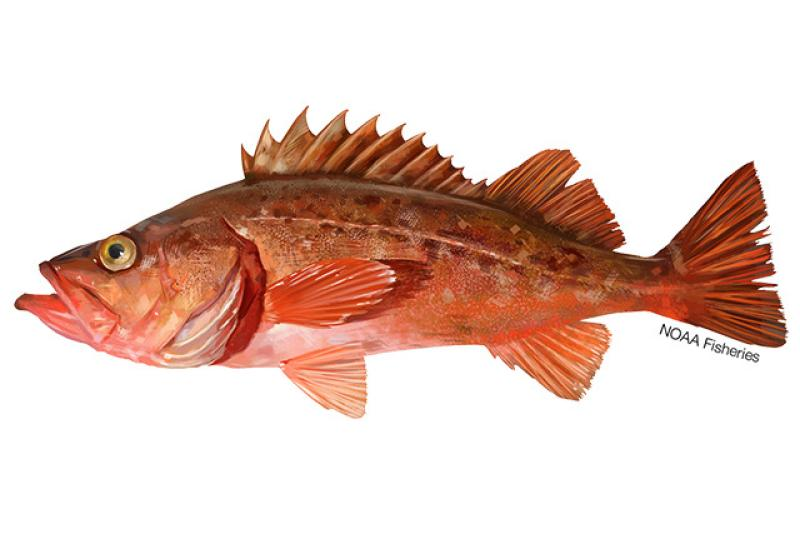
The Rockfish Recruitment and Ecosystem Assessment Survey (RREAS) is a long-running survey of juvenile rockfish, their physical environment, and their predators along the US west coast. The survey is vitally important for understanding the population dynamics of economically and culturally important species, such as bocaccio. RREAS data inform fishery management decisions to protect threatened populations while supporting California’s coastal economy. For more information about RREAS, see their Story Map.
The RREAS has run almost every spring for over 40 years. The “almost” qualifier is necessary because the COVID-19 pandemic greatly reduced survey effort in 2020. NOAA scientists used linear regression to fill the gap in their dataset with a proxy measurement: diets of common murres.
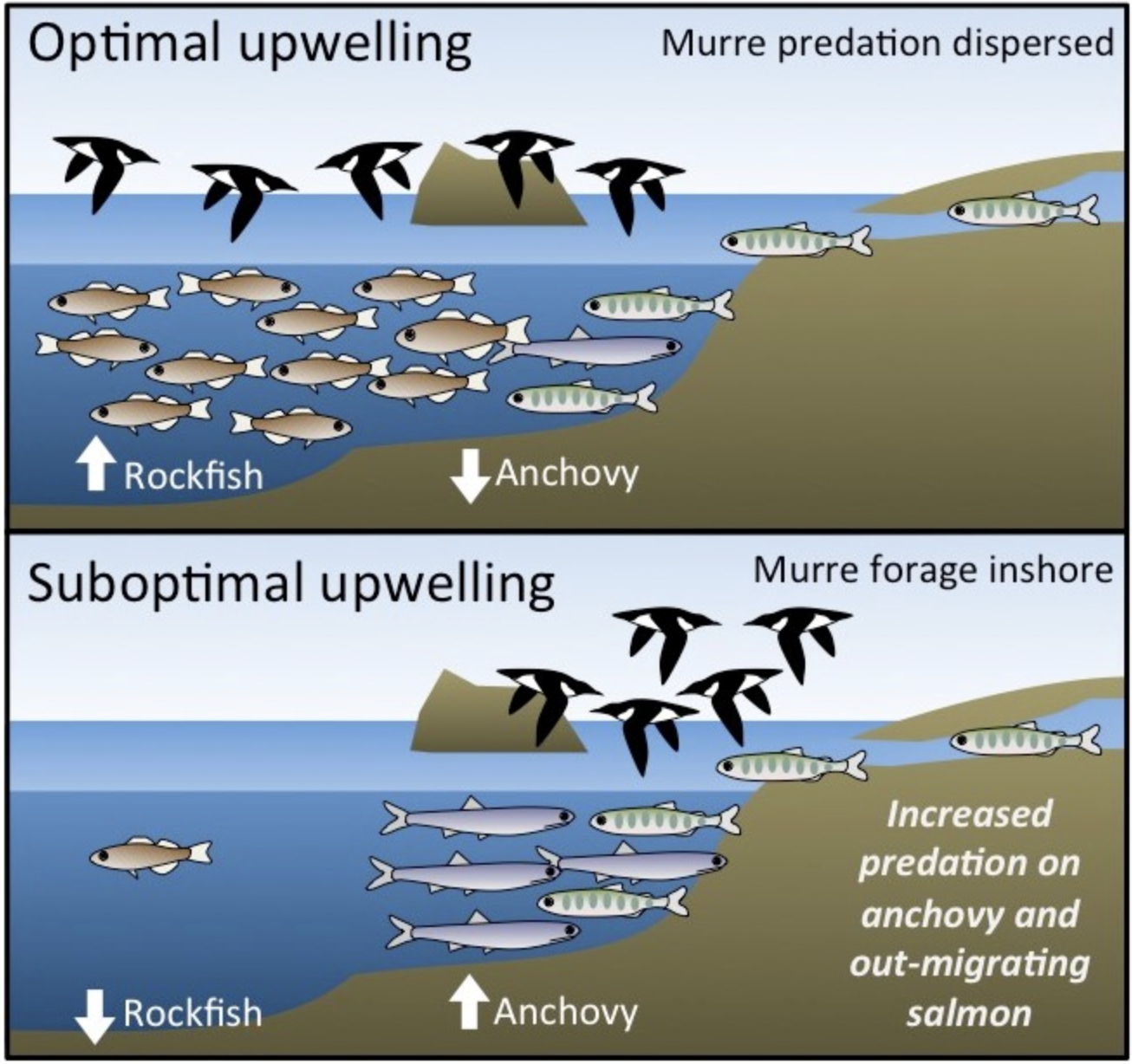
The common murre is a seabird that breeds in large numbers off the coast of California. In spring, pairs of murres raise one chick by bringing it juvenile fish, including rockfish, anchovy, and salmon. The composition of common murre diets on the Farallon Islands (~30 miles west of San Francisco) has been recorded by biologists with Point Blue Conservation since the 1970s.
Explore the data
Read the data from the rreas.csv file and create a scatter plot relating fish abundance indices to common murre diet.
rreas_murres <- read_csv("data/rreas.csv")Q6: Which variables did you choose for the x- and y-axis? What does this mean for the purpose of your model?
Fit the model
Fit a model that predicts the RREAS rockfish abundance index from the fraction of rockfish in common murre diets.
Interpret the model
Find the \(R^2\) value for your model.
Q7: What does the R2 value tell you about the utility of your model for filling in the survey gap?
Extract the estimated coefficients (\(\hat \beta_0, \hat \beta_1\)) and standard deviation (\(\hat \sigma\)) from the model.
Q8: In plain language, what do the coefficients and standard deviation of the model represent?
Say it’s 2020 and the RREAS has largely been canceled. You ask Point Blue to share their common murre diet data with you and they say it was 32.8% juvenile rockfish. Estimate the predicted value of the juvenile rockfish abundance index.
Q9: What did you predict the juvenile rockfish abundance index was in 2020?
Q10: Your prediction is the most likely outcome, but the actual index won’t take that value exactly. How would you estimate an interval that you could confidently say probably contains the actual index?
Recap
In this lab, you fit linear regression models to one predictor and one response variable. You used statistical notation to describe the model, which makes two things unambiguous.
- It shows the relationship between the predictor, model coefficients, and the expected value of the response for a given value of the predictor.
- It says the observed response values are normally distributed around the expected value, with a standard deviation of \(\sigma\).
In future weeks, we’ll build on this foundation to make more complicated models. You’ll add additional predictors, transform parameters to introduce non-linearity, and use non-normal random variables to model other types of responses.