EDS 222: Statistics for Environmental Data Science

Learning objectives

In today’s lab you will…

Use mathematical models to test hypotheses
Use mathematical models to construct confidence intervals
Compare mathematical and randomization approaches to inference

library(tidyverse)
theme_set(theme_classic(14))
set.seed(123)

Mathematical models

This lab will repeat the inferences you conducted in last week’s lab, using mathematical models instead of randomization. Let’s recall our data from last week. You’ll need to copy the data file to your week5/data directory.

restoration <- read_csv("data/eelgrass.csv",
                        show_col_types = FALSE)
ggplot(restoration, aes(treatment, fill = success_fct)) +
  geom_bar() +
  scale_fill_manual(values = c("firebrick", "cornflowerblue")) +
  labs(x = "Restoration method",
       y = "Sites",
       fill = "Outcome") +
  theme(legend.position = "inside",
        legend.position.inside = c(1, 1),
        legend.justification = c(1, 1))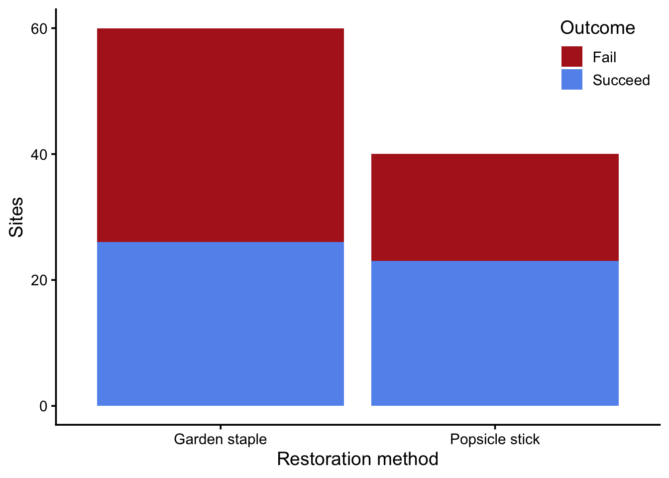

Figure 1: Success of eelgrass restoration plots by restoration method.

Hypothesis test

Once again, we want to know if the popsicle stick method works better for restoration than garden staples. This is a “yes/no?” question, so we’re conducting a hypothesis test. Instead of using permutation to estimate our sampling distribution, we will assume the sampling distribution is normally distributed. Under the null hypothesis (i.e., no difference in proportions), we make this assumption:

\[ \begin{align} \hat{p_2} - \hat{p_1} &\sim Normal(0, SE(\hat{p})) \\ \hat{p} &= \frac{x_1 + x_2}{n_1 + n_2} \\ SE(\hat{p_2} - \hat{p_1}) &= \sqrt{\hat{p} (1 - \hat{p}) (\frac{1}{n_1} + \frac{1}{n_2})} \\ \end{align} \]

Note

This math describes the assumptions of the null hypothesis for a difference in proportions. The key points are:

The distribution of the statistic (\(\hat{p_2} - \hat{p_1}\)) follows a normal distribution (i.e., the shape of the sampling distribution).
We assume the mean of the sampling distribution is 0, because this is the null hypothesis.
The standard error of the sampling distribution is based on the POOLED proportion because we’re assuming no difference between the proportions.

This is how you would have tested your hypothesis using permutation:

Identify the STATISTIC
State your NULL and ALTERNATIVE hypotheses
Calculate the OBSERVED statistic
Estimate the NULL DISTRIBUTION
Calculate P-VALUE
Compare p-value to CRITICAL THRESHOLD

Using a mathematical model, you modify step 4. Instead of using randomization to estimate the null distribution, you use a normal variable. The following questions walk you through the steps. Note: many of these steps are exactly the same as last week’s lab.

Identify the statistic

Q1: What is the appropriate statistic for this question?

Difference in proportions

State your null and alternative hypotheses

Q2: What are your null and alternative hypotheses?

H0: There’s no difference in outcome between garden staple and popsicle stick methods.

HA: The popsicle stick method is more likely to succeed than the garden staple method.

Calculate the sample statistic

Q3: How would you calculate the statistic for the sample?

Call the variable diff_props.

success_props <- restoration %>% 
  group_by(treatment) %>% 
  summarize(prop_success = mean(success))

diff_props <- success_props$prop_success[2] - success_props$prop_success[1]

diff_props

[1] 0.1416667

Estimate the null distribution

Q4: What’s the standard error of the sample’s statistic?

# p_hat is the POOLED proportion, i.e. the overall proportion of success
p_hat <- sum(restoration$success) / nrow(restoration)

# n's are the number of observations in each treatment
# n1: number of garden staple observations
# n2: number of popsicle stick observations
n1 <- sum(restoration$treatment == "Garden staple")
n2 <- sum(restoration$treatment == "Popsicle stick")

se_p_hat <- sqrt(p_hat * (1 - p_hat) * (1 / n1 + 1 / n2))

If you calculated se_p_hat correctly, the following figure should depict the PDF of the null distribution. It should be a normal variable with mean equal to 0 and standard deviation equal to the standard error of \(\hat p\).

null_dist <- tibble(
  diff_prop = seq(-0.4, 0.4, length.out = 1000),
  density = dnorm(diff_prop, mean = 0, sd = se_p_hat)
)
 
ggplot(null_dist, aes(diff_prop, density)) +
  geom_line(color = "cornflowerblue", linewidth = 2) +
  geom_vline(xintercept = diff_props, color = "firebrick", linewidth = 2)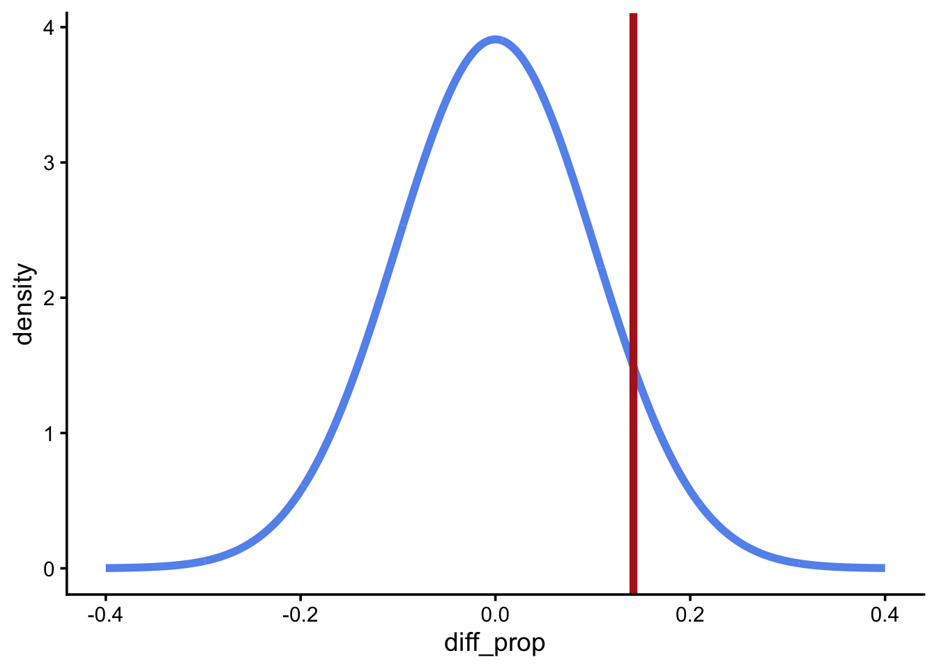

Calculate the p-value

Use the pnorm() function to get the area under the curve of a normal distribution.

Tip

By default, pnorm() will tell you the area under the curve to the left of a value. Since we want the area to the right of the observed statistic, set lower.tail to FALSE.

Q5: Fill in the blanks to calculate the p-value

p_val <- pnorm(diff_props, mean = 0, sd = se_p_hat, lower.tail = FALSE)
p_val

[1] 0.08251953

Compare p-value to critical threshold

Q6: How does your p-value compare to a critical threshold \(\alpha=0.05\)? How would you interpret that?

The p value is greater than the critical threshold, so we fail to reject the null hypothesis. Our data are not consistent with the hypothesis that the popsicle stick method leads to success more often than the garden staple method.

Confidence interval

Now we want to estimate how differently the popsicle stick and garden staple methods perform. This is a “how much?” question, so we’re constructing a confidence interval. Instead of using bootstrapping to estimate our sampling distribution, we will assume the sampling distribution is normally distributed. We make this assumption:

\[ \begin{align} \hat{p_2} - \hat{p_1} &\sim Normal(p_2 - p_1, SE(\hat{p_2} - \hat{p_1})) \\ SE(\hat{p_2} - \hat{p_1}) &= \sqrt{\frac{\hat{p_1}(1 - \hat{p_1})}{n_1} + \frac{\hat{p_2}(1 - \hat{p_2})}{n_2}} \\ \end{align} \]

Note

This math describes the assumptions of constructing a confidence interval for a difference in proportions. The key points are:

The distribution of the statistic (\(\hat{p_2} - \hat{p_1}\)) follows a normal distribution (i.e., the shape of the sampling distribution).
We assume the mean of the sampling distribution is the population parameter (\(p_2 - p_1\)).
The standard error of the sampling distribution is based on the two samples’ proportions, rather than pooling them, because we’re assuming there’s a difference between the proportions.

This is how you would have built a confidence interval using bootstrapping:

Identify the STATISTIC
Substitute sample for population and draw BOOTSTRAP SAMPLES
Estimate the BOOTSTRAP DISTRIBUTION of the statistic
Construct the CONFIDENCE INTERVAL

Using a mathematical model changes how steps 2 and 3 work, with the same goal of estimating the sampling distribution. Instead of using randomization to draw bootstrap samples, you use a normal variable. The procedure works like this:

Identify the STATISTIC
Calculate the STANDARD ERROR of the statistic
Construct the CONFIDENCE INTERVAL using a normal variable

The following questions walk you through the steps.

Identify the statistic

Q7: What is the appropriate test statistic for this question?

Difference in proportions

Calculate the standard error

Q8: Fill in the blanks below to calculate the standard error of the statistic

Note

Remember that the standard error is going to differ between hypothesis testing and confidence intervals. Hypothesis testing begins by assuming the null hypothesis is true, so the standard error describes a scenario where there are no differences (\(p_2=p_1\)). Confidence intervals assume the difference is real, so the standard error comes from a different scenario (\(p_2 > p_1\)). Hence the difference in equations.

# Calculate the proportions of the two treatments
# Let treatment 1 be "Garden staple"
p_hat1 <- mean(restoration$success[restoration$treatment == "Garden staple"])
# Let treatment 2 be "Popsicle stick"
p_hat2 <- mean(restoration$success[restoration$treatment == "Popsicle stick"])

# n1 and n2 remain the same from before

# Calculate standard error
se_diff_props <- sqrt(p_hat1 * (1 - p_hat1) / n1 + p_hat2 * (1 - p_hat2) / n2)
se_diff_props

[1] 0.1010048

If you calculated se_diff_props correctly, the following figure should depict the PDF of the sampling distribution. It should be a normal variable with mean equal to the observed statistic in the sample and standard deviation equal to the standard error.

sampling_dist <- tibble(
  diff_prop = seq(-0.2, 0.5, length.out = 1000),
  density = dnorm(diff_prop, mean = diff_props, sd = se_diff_props)
)
 
ggplot(sampling_dist, aes(diff_prop, density)) +
  geom_line(color = "cornflowerblue", linewidth = 2) +
  geom_vline(xintercept = diff_props, color = "firebrick", linewidth = 2)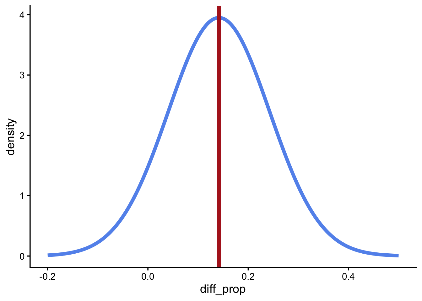

Construct the confidence interval

Using bootstrapping, you constructed the confidence interval using the 2.5% and 97.5% quantiles of the bootstrapped sampling distribution. Using the mathematical model, you use the function qnorm(). Whereas pnorm() returns the area under the curve, qnorm() tells you what value corresponds to a given area. In other words, they’re inverses of each other.

If you wanted to shade in the middle 95% of the area in Figure 3, qnorm() would tell you the left and right boundaries.

Q9: Fill in the blanks to use qnorm() in constructing the confidence interval.

diff_props_ci <- qnorm(c(0.025, 0.975), mean = diff_props, sd = se_diff_props)
diff_props_ci

[1] -0.05629908  0.33963242

Q10: How would you interpret this confidence interval

We are 95% confident the true difference in proportions falls between -0.06 and 0.34.

Comparing mathematical and randomization approaches

Q11: What are permutation tests and mathematical models both trying to estimate for hypothesis tests?

The sampling distribution of the statistic assuming the null hypothesis is true.

Q12: What are bootstrapping and mathematical models both trying to estimate for confidence intervals?

The sampling distribution of the statistic assuming the difference is real.

Q13: What area under the curve is relevant to hypothesis tests? What R function calculates it for a mathematical model?

The area of the null distribution more extreme than the observed value. pnorm()

Q14: What area under the curve is relevant to confidence intervals? What R function calculates it for a mathematical model?

The middle 95% of the area under the sampling distribution. qnorm()